A few days later than planned (sorry about that), but here we go with part 2 (Part1) and the demodulation/analysis part.
Initial Analysis
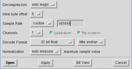
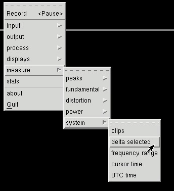
To analyse a captured signal, the tool baudline seems to be the best way at the moment. So we open it with the following options and have a closer look (ContextMenu->Input->Open file):
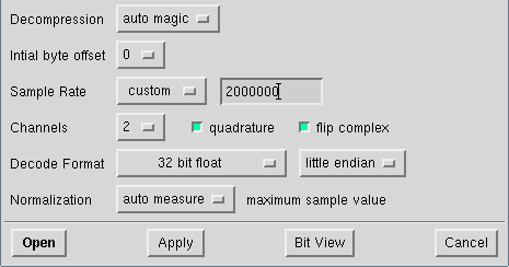
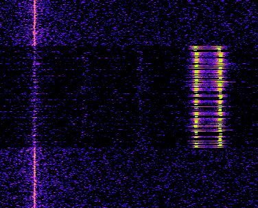
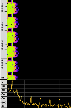
After using the open button, you should be able to see something similar to this:
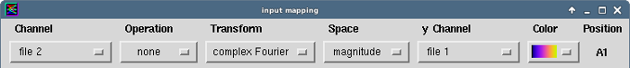
There might be some differences in the colors and the amount of noise. These settings can be simply adjusted by using, on the one hand, the ContextMenu->Input->Channel Mapping, and set it e.g. like this:
And on the other hand, by adjusting the noise (ContextMenu->Input->Color aperture), e.g. like this:
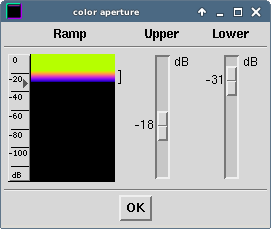
The ideal values for the color aperture depend hardly on the signal strength and almost always needs some tweaking. Besides, I wouldn’t recommend adjusting the color aperture AFTER zooming in the relevant part (by using ALT or CTRL + mousewheel or arrowUp/arrowDown):
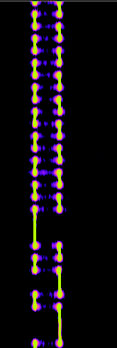
What now can be seen is in the beginning a long sequence of short impulses with always the same length, switching between two different frequencies and afterwards also some longer impulses. At this point, we can make two assumptions:
- The many short impulses in the beginning are most probably some kind of preamble, which helps the receiver of the signal to synchronize its internal clock
- The transported information are likely modulated using a form of FSK (Frequency-shift keying), presumably binary FSK (one frequency means 0, the other 1)
Before now trying to demodulate bits and bytes (especially, because this process takes some time), I would first proceed with some further manual analysis, regarding some relevant points:
- Is the signal in any way changing when using the same button over and over again?
- How does the signal change for different buttons from the remote control?
- How does a signal look like, when the motion detector comes into play?
Depending on the length of a whole signal, a manual comparison might be pretty exhausting. One quick approach to get a first impression would be simply having a look at the beginning of the signal (right after the long sequence of short impulses = preamble) a part in the middle and at the end.
Another way would be to count the number of long and/or short impulses on each frequency.
A more complete comparison is to write down the sequence for each frequency (e.g. freq1: short short long short long… freq2: long long short), and compare this with another signal (e.g. by simply putting the output in files and using diff).
The fact, that in our case
- the very beginning of the signal seems always to be the same,
- the middle part only changes from remote control to motion detector and
- the end part changes for different buttons
gives us a good clue as to what we should expect from a successful demodulation.
Demodulation
As we now gathered enough information, we can start trying to build a demodulator. The first step in this process is to center the relevant signal on the base frequency (in the context of gnuradio) and filter irrelevant signals out.
It is recommended to first shift the signal to the center, using “Multiply” and “Signal Source”:
Afterwards, everything else can be filtered, using a “Low Pass Filter”. Don’t use a too low Transition width as it exhausts the CPU. The usage of a decimation of 11 in this example additionally gets rid of unimportant data. Decimation is the process of reducing the sample rate (e.g. take one and throw the rest away). In general, it should be set as high as possible, so the demodulation process costs less CPU, but shouldn’t be set over a certain level (see CAUTION part below). The last step I usually like to do, is to add a “Power squelch”, which drops every peak, which is below a certain dB level (this can become important in the final demodulation step). The final result looks like this:
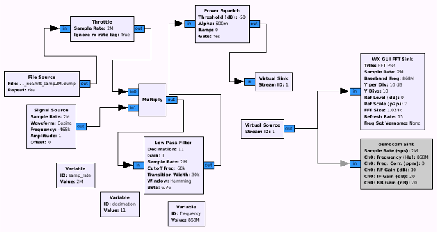
CAUTION!!! If decimation is set too high, it may have unexpected side effects, like the output produces 0 instead of 1 and vice versa. So, the final sample rate (calculated by dividing capture-sample-rate by decimation) must NOT be less than the bandwidth left from the low pass filter (cutoff of 60k times 2 (= 120KHz)). So:
2MHz / 11 = 181Khz
As 181KHz is greater than 120KHz, a decimation of 11 is OK.
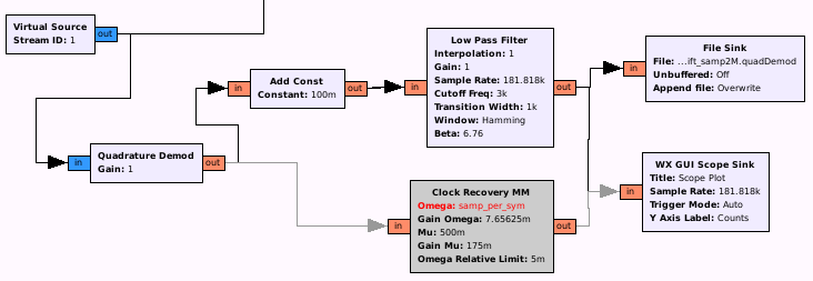
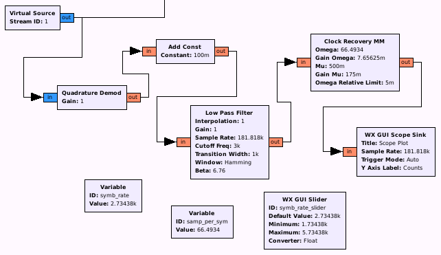
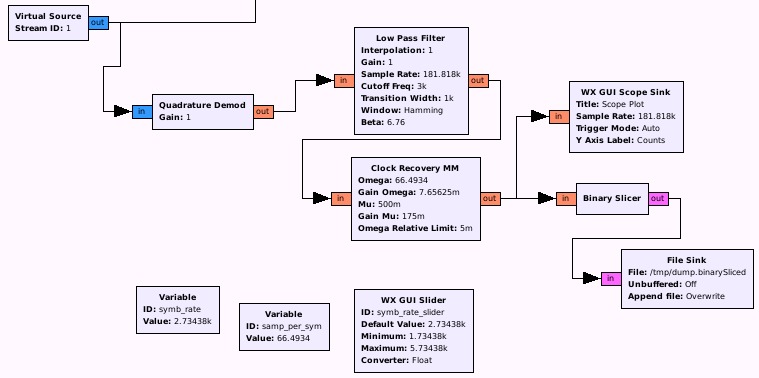
The next step is to first convert the complex input into float with “Quadrature Demod” and a Gain of 1, and afterwards use “Clock Recovery MM” to synchronise gnuradios clock with the clock of the sender (using the preamble). The tricky part here is to get the correct value for Omega on the Clock Recovery MM. This value is normally samples-per-symbol and is in general calculated by the following formula:
samp_per_sym = (sample_rate/decimation) / symb_rate
As the only part we don’t know now is the symbol rate, we shortly deactivate the clock recovery and focus on the output of the quad demod.
NOTE!!! For the Scope sink at the end, you need samp_rate/decimation (2MHz/11) as the sample rate.
The first step, in order to get the symbol rate, is to center the peaks at zero line (if not already, use the “add const”) and to nicely shape the waves (if not already: use again a low pass filter, if there is noise).
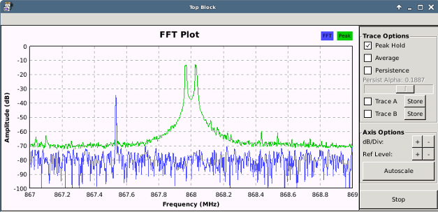
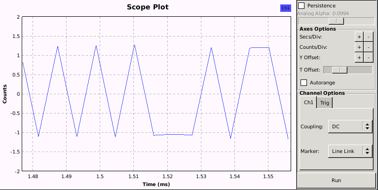
The first screenshot shows the centered signal after quad demod without additional low pass filtering:
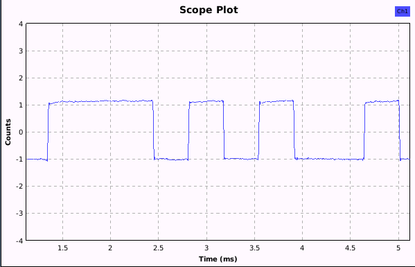
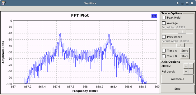
The second screenshot shows the same signal after using an additional low pass filtering:
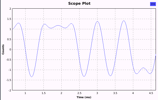
Note, that the autorange option has been deactivated and the secs/div and count/divs values adjusted.
Note: In this case, the demodulation would also have worked without the low pass filtering (shaping).
As can be seen in the flow graph, there is also a file sink at the end, as the next step would be to open the output again with baudline (note again the decreased sample rate: capture-sample-rate / decimation):
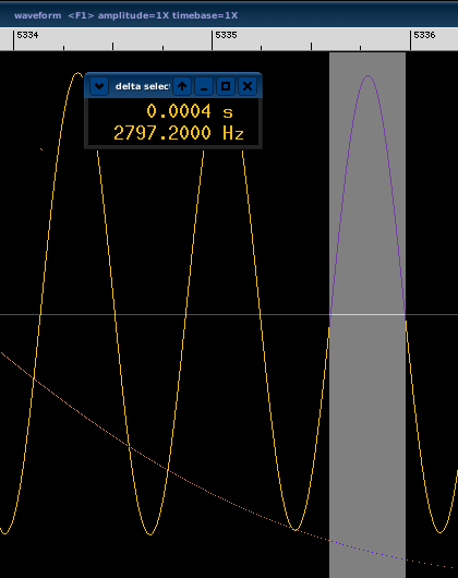
The next step is to get the symbol rate, which is the number of crossings of the zero line, or the number of upper and lower peaks in a given time. Baudline offers an easy to read way to gather this value, named DeltaView. So we open up the waveform view, point the synchronization signals, and open the delta view:
The last step is to simply mark (as accurate as possible) the wave like in this picture and read the symbol rate:
So we are now ready to go back to our flow graph and to add some necessary variables, like symb_rate and samp_per_sym and place samp_per_sym in our now activated Clock recovery block:
As you can see, I added a slider for the symbol rate, as this value normally needs a try and error approach to get right (in my case, the original value of 2740 seems pretty good, but in the end, after decoding 500 packets (see last part of this chapter), a symbol rate of 2734,38 Hz does produce a more stable output (with 2740, 3 out of 500 decoded packets had a slightly different value)). The result you want to see should look in this case something like that:
Note, that the autorange option has been deactivated and the secs/div and count/divs values adjusted.
At this point, we are finally ready to try to get bits out of those peaks, so we add a binary slicer and dump the output in a file:
When we now run this flow graph for a few seconds, we should have an output file with some data in it:
xxd /tmp/dump.binarySliced

0000000: 0000 0001 0100 0100 0100 0100 0100 0100 ................

0000010: 0100 0100 0100 0100 0100 0100 0100 0100 ................

0000020: 0100 0100 0100 0100 0100 0100 0000 0100 ................

0000030: 0101 0001 0101 0001 0001 0000 0100 0101 ................

0000040: 0000 0101 0001 0101 0101 0101 0101 0001 ................

0000050: 0001 0100 0100 0000 0001 0100 0000 0001 ................

0000060: 0001 0101 0100 0100 0001 0001 0101 0001 ................

0000070: 0001 0001 0001 0001 0001 0001 0001 0001 ................

0000080: 0001 0001 0001 0001 0001 0001 0001 0001 ................

0000090: 0001 0001 0000 0001 0001 0100 0101 0100 ................

00000a0: 0100 0100 0001 0001 0100 0001 0100 0101 ................

00000b0: 0101 0101 0101 0100 0100 0101 0001 0000 ................

00000c0: 0000 0101 0000 0000 0100 0101 0101 0001 ................

00000d0: 0000 0100 0101 0100 0100 0100 0100 0100 ................

00000e0: 0100 0100 0100 0100 0100 0100 0100 0100 ................

00000f0: 0100 0100 0100 0100 0100 0100 0100 0000 ................

...
This doesn’t look bad. What we now try to find is the preamble of multiple 1,0 sequences and we can spot that for example in row 0000070 (Note: a one is 01 and zero is 00). To verify the correct demodulation, we should now compare bits after the preamble with the sequence from the baudline view at the beginning. In this case we get 0,0,0,1,0,1,1,0,1,1,… in line 0000090, which perfectly correlates with the signals from baudline, when you interpret the higher (right) frequency as a 1 and the lower (left) frequency as 0.
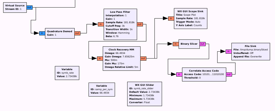
As you can see, we get also some noise (e.g. in the beginning), which we are not interested in. So the next step would be to add a marker at each packet beginning, so that we can spot easily different packets. The block “Correlate Access Code” does exactly that for us. The only necessary part to configure here is the sequence which identifies a new packet. For our example, this sequence can be expressed in python syntax like this:
"10" * 10 + "0010110111010100"
It is a string concatenation of the preamble (1,0 times 10) and 16 following bits, which are most probably the packet frame delimiter.
After applying this to our flow graph, we hopefully get now some markers in our output:
xxd /tmp/dump.binarySliced

0000000: 0000 0000 0000 0000 0000 0000 0000 0000 ................

0000010: 0000 0000 0000 0000 0000 0000 0000 0000 ................

0000020: 0000 0000 0000 0000 0000 0000 0000 0000 ................

0000030: 0000 0000 0000 0000 0000 0000 0000 0000 ................

0000040: 0000 0001 0100 0100 0100 0100 0100 0100 ................

0000050: 0100 0100 0100 0100 0100 0100 0100 0100 ................

0000060: 0100 0100 0100 0100 0100 0100 0000 0100 ................

0000070: 0101 0001 0101 0001 0001 0000 0300 0101 ................

0000080: 0000 0101 0001 0101 0101 0101 0101 0001 ................

0000090: 0001 0100 0100 0000 0001 0100 0000 0001 ................

00000a0: 0001 0101 0100 0100 0001 0001 0101 0001 ................

00000b0: 0001 0001 0001 0001 0001 0001 0001 0001 ................

00000c0: 0001 0001 0001 0001 0001 0001 0001 0001 ................

00000d0: 0001 0001 0000 0001 0001 0100 0101 0100 ................

00000e0: 0100 0100 0003 0001 0100 0001 0100 0101 ................

00000f0: 0101 0101 0101 0100 0100 0101 0001 0000 ................
Note the 03 in line 0000070, right after our 1,0 sequence (in this case, 0100, not 0001 as before) and the 16 bits packet delimiter.
At this point we are almost done, except for forming those bits into something more readable. A little script which searches for the markers and converts the byte-coded bits into bytes is sufficient. After some try and error with some outputs, or by manually counting, we get a packet size of 6 bytes (without the preamble and packet delimiter). So let’s try that:
packet 0

HEX: b37fd68617a5

RAW: (non printable characters)
packet 1
HEX: b37fd68617a5
RAW: (non printable characters)
packet 2
HEX: b37fd68617a5
RAW: (non printable characters)
...
Packet Format
After processing signals for different functions with our demodulation (unlock/lock on the remote control, activation of the motion detector, …), the following packet format can be extracted:
+--------------------------------------------+-----------------+-----------------+---------------------+-------------------------+
|                       |                    |                 |                 |                     |                         |
|       Preamble        |     Start of       |    Device ID    |  Unknown Part/  |      Command        |         Checksum        |
|                       |  packet delimiter  |                 |   Future Use    |                     |                         |
|                       |                    |                 |                 |                     |                         |
+-----------------------+--------------------+-----------------+-----------------+---------------------+-------------------------+
|                       |                    |                 |                 |                     |                         |
|  40 bits; "1,0" * 20  |  16 bits;  0x2dd4  |    24 bits      |  8 bits; 0x86   |  8 bits; e.g. 0x17  |  8 bits; byte wise add  |
|   or 0xaaaaaaaaaa     |                    |  e.g. 0xb37fd6  |                 |   for unlocking     |  of id,unknown,command  |
|                       |                    |                 |                 |                     |  thx to M. Ossmann ; )  |
+-----------------------+--------------------+-----------------+-----------------+---------------------+-------------------------+
Possible commands
When using different functions from the remote control, we are easily able to spot the different codes:
0x17 = Unlock

0x1d = Lock Home (Doesn't make a phone call)

0x1b = Lock with Call

0x1e = SOS (starts immediately the alarm)
Coming from a motion detector:
0x0f = Motion detected (starts count down)
So that’s it for the second part. The next and last part will be focusing on the modulation process (e.g. convert a specific command into a signal). So again, stay tuned ; )
Regards,
Frank